The science behind the poem

Mr. In Situ stands for surface measurements such as the record at Mauna Loa, Hawaii, which Charles David Keeling started in 1958. OCO is NASA’s Orbiting Carbon Observatory-2, which measures CO₂ around the globe but cannot see through clouds. The slow trains of the stratosphere stand for how long air can stay up there before it comes back down.

For the science, see Pandey et al. (2024), AGU Advances, which compares the sampling errors of satellite and in situ approaches. More on this work is in Research.

Building the adjoint of a big atmospheric transport model — the thing you need to turn satellite measurements into emission estimates — was a rite of passage, talked about the way climbers talk about a summit. It could eat a year or two of someone’s PhD. People wrote papers just about how to write the adjoint code (Giering & Kaminski, 1998). Whole model versions were named after it: the GEOS-Chem adjoint (Henze et al., 2007), the TM5 four-dimensional variational system (Meirink et al., 2008).

It ate the first six months of mine. I spent them learning to build adjoints by hand, and being quietly floored that the recipe worked at all: apply a fixed set of rules, mechanically, backwards through every line of your model, and out falls the gradient of your cost with respect to every input. Not an approximation — the exact gradient, to floating-point precision. A physical simulation could be made to hand you its own exact sensitivities, if you were only disciplined enough about the bookkeeping. And it did not end with the PhD: through my first postdoc I was still in the thick of it — squeezing an order-of-magnitude speed-up out of the TM5-4DVAR variational inversion system (Pandey et al., 2022), among other variational-inversion work.

Then differentiable programming showed up and quietly deleted the hard part.

If your forward model is written in a framework like JAX, the adjoint is already there. You do not derive it. You do not hand-code it. You call jax.grad, and the framework walks backward through your model and hands you the gradient. The thing that used to cost a PhD now costs one line.

Everything below is built from toy models small enough to run on a laptop — two of them you can play with right here on the page.

Why anyone wants an adjoint in the first place

Start with the picture that pays for a lot of Earth-observing satellites.

A spectrometer in orbit — TROPOMI, GOSAT, OCO-2 — measures how much methane or CO₂ sits in a column of air. What we actually want is not the concentration. It is the emissions: which well, which wetland, which city, leaking how much (Jacob et al., 2016).

Between the two sits a forward model:

emissions  ──►  [ atmospheric transport + chemistry ]  ──►  concentrations
   (what we want)                                            (what we see)

The inverse problem is to run that arrow backwards: find the emissions that, pushed through the model, best reproduce what the satellite saw. In practice you never invert the arrow directly. You define a mismatch — a scalar cost that measures how far the model is from the observations (plus a term keeping you near a prior) — and you slide the emissions downhill until it is small. This is the heart of variational inverse modelling, from global CO₂ budgets to satellite methane — with some of the first global CO₂ flux inversions from GOSAT total-column retrievals (Basu et al., 2013) sitting in between. The textbook, if you want one, is Enting (2002).

To slide downhill you need the gradient: how does the mismatch change if I nudge each emission parameter? And here is the catch that makes or breaks the whole enterprise. A real flux inversion does not have four unknowns. It has emissions on a grid — thousands to millions of them. You need the derivative of one number (the mismatch) with respect to all of them.

There are two ways to get it.

• Finite differences. Nudge one parameter, re-run the whole model, see how the mismatch moved. Repeat for every parameter. For P unknowns that is about 2P full model runs. For a million-parameter inversion, that is a non-starter — you would be re-running a chemistry-transport model a million times just to take one step downhill.
• The adjoint. Run the model forward once, then run a single backward pass that propagates the sensitivity of the mismatch back through every operation, accumulating the derivative with respect to every parameter along the way. One forward pass, one backward pass, the entire gradient — almost regardless of how many unknowns.

That backward pass is the adjoint. If you have ever trained a neural network, you already know it under a different name: backpropagation. Reverse-mode automatic differentiation, the adjoint method, and backprop are the same idea wearing three different lab coats (Errico, 1997 is still the friendliest one-page explanation for atmospheric scientists).

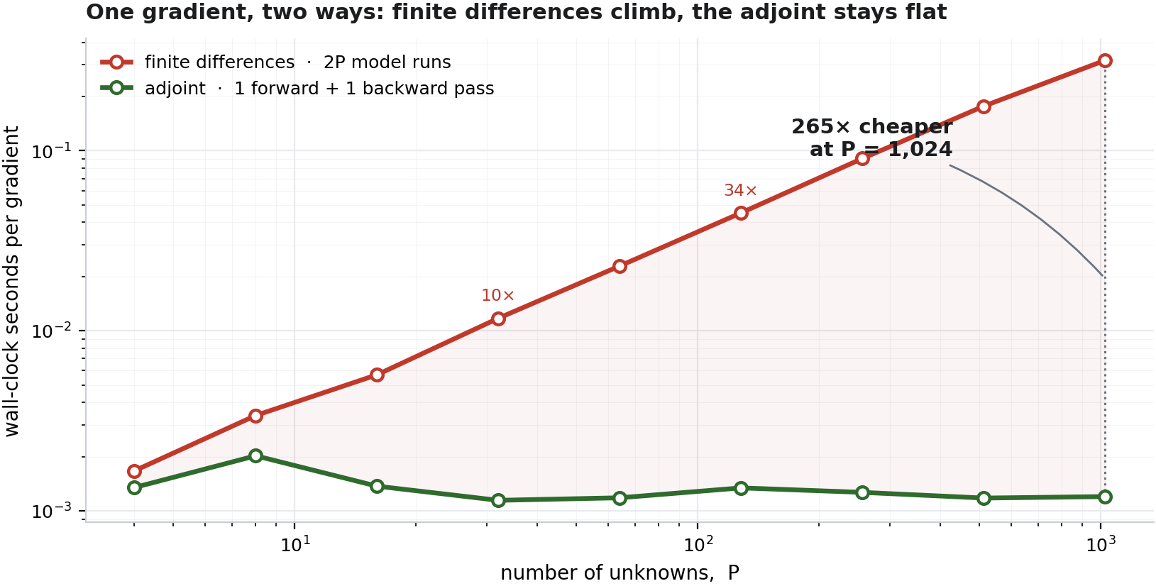
Here is that trade-off, measured on a toy chemistry model — finite differences climb with every unknown you add, while the adjoint stays almost flat:

Finite differences re-run the whole model twice per unknown; the adjoint gets the entire gradient in one backward pass, for roughly the same price no matter how many unknowns there are. By 1,000 it is ~265× cheaper — and the gap keeps widening.

At a hundred thousand parameters, that gap is the difference between “runs overnight” and “never finishes.”

The free lunch, in one line

Here is the part that still feels like cheating.

Take the simplest possible physical model — 1-D diffusion, heat (or a tracer) spreading along a line:

du/dt = kappa * d²u/dx²

with a single unknown, the diffusivity kappa. Write the time-stepper in JAX, make some synthetic “observations” with a known kappa_true, and define the mismatch:

import jax, jax.numpy as jnp

def forward(kappa):
    u = u0
    for _ in range(n_steps):                 # explicit diffusion step
        u = u + kappa * dt/dx**2 * (jnp.roll(u,1) - 2*u + jnp.roll(u,-1))
    return u

def loss(kappa):
    return jnp.mean((forward(kappa) - u_obs)**2)

grad_loss = jax.grad(loss)      # <-- this is the discrete adjoint. that's it.

(One vocabulary note before anything else: the loss in that code is exactly what the inverse-modelling literature calls the cost function — the single number you minimise. Same object, two dialects; I’ll use the words interchangeably.)

jax.grad(loss) is the adjoint of your time-stepping model. Not an approximation of it — the exact derivative of the numerical code you wrote, assembled by differentiating every operation in reverse, at least for the parts of the model JAX can trace (more on where that breaks below). Conceptually:

forward:    kappa ──► diffusion steps ──► final state ──► loss
backward:   d(loss) ──► d(final state) ──► back through every time step ──► d(loss)/dkappa

No adjoint model was written. Feed that gradient to an optimizer and the inverse problem just… solves:

true kappa:            0.035000
initial guess:         0.006000
recovered kappa:       0.035513      (1.5% off, from a 6× wrong start)

Twenty years ago, that would have been a week of careful calculus and debugging. Now it is a function call.

A cartoon of a real methane inversion

One unknown is a party trick. Let’s make it look a little more like the day job.

I built a two-box atmospheric chemistry model: a “northern” box and a “southern” box that exchange air, each carrying three tracers — CH₄, CO, and NOₓ. The chemistry is deliberately nonlinear: CH₄ and CO are destroyed by the hydroxyl radical OH, and OH itself depends on how much CH₄, CO, and NOₓ are present. (That coupling — methane’s lifetime depending on the very air it sits in — is a real headache for explaining methane’s ups and downs; Bousquet et al., 2006.)

Then I hid the answer. I picked four “true” emission scale factors, generated synthetic CH₄ and CO observations over five years, and asked the inversion to recover the emissions it was never told:

control        true      recovered
CH4 north      1.3000     1.2999
CO  north      0.7000     0.7000
CH4 south      0.7500     0.7501
CO  south      1.4000     1.4000

Four decimal places — in this clean, noise-free synthetic case — from one scalar mismatch and its adjoint gradient, through a nonlinear coupled-chemistry model. Same one line, jax.value_and_grad(loss), doing the work. Recovering several coupled tracers at once from column measurements is exactly the shape of a real satellite inversion: the very first paper of my PhD was a joint CH₄/CO₂ column inversion of much the same shape (Pandey et al., 2015). It is the same machinery behind today’s operational methane and CO₂ flux estimates (Meirink et al., 2008; Chevallier et al., 2005).

Okay, you have the gradient. Now what do you do with it?

A gradient tells you which way is downhill. It does not tell you how big a step to take, and this is where a lot of grad-student hours quietly disappear.

The plainest choice is a first-order optimizer — Adam, the workhorse from deep learning — which only ever looks at the gradient. It works, but it can be slow, wandering down long narrow valleys taking cautious steps.

The alternative is to use curvature — second-derivative information about how the landscape bends. Two classic moves from the inverse-problems world:

• Gauss-Newton / Levenberg-Marquardt approximates the curvature from the Jacobian of the residuals (JᵀJ). It is the default for smooth least-squares problems for a reason.
• Full Newton uses the exact Hessian — which JAX will hand you for a small problem, jax.hessian(loss) (at real scale you never form it; you use Hessian-vector products instead).

Get a feel for the difference on the classic test valley below: gradient descent only sees the slope and zig-zags for thousands of steps; curvature cuts across in a dozen. Drag the start point and race them.

The same pattern holds on our actual two-box chemistry model: with a nonlinear penalty added, Adam grinds through about 180 iterations to settle, while Gauss-Newton — using curvature from the residual Jacobian — gets there in 7.

And here is the part that should make a carbon-cycle person sit up: the curvature you compute to go fast is the same curvature you need for error bars. For Gaussian errors and a linear approximation near the solution, the posterior covariance — your uncertainty on the recovered emissions — is

posterior covariance  ≈  ( Jᵀ R⁻¹ J  +  B⁻¹ )⁻¹

that same JᵀJ-shaped object, built from the prior (B) and observation (R) error covariances. In our field a flux estimate without an uncertainty is not a result — it is a rumour. So the method that converges fastest is also the one that tells you how much to trust the answer. You rarely get to have both; here you do.

An aside for the inversion crowd. That Gauss-Newton Hessian A = JᵀR⁻¹J + B⁻¹ is doing double duty: its inverse is the posterior covariance, and that same inverse maps the gradient straight to the answer in a single Newton step, x* = x₀ − A⁻¹g — from a starting guess x₀ to the optimum x*, with g the gradient (a quadratic cost has constant curvature, so one step lands it). So why do operational CH₄/CO₂ inversions grind through hundreds of conjugate-gradient iterations instead of solving in one shot? Because that gradient is only g = A(x − x*) — the Hessian times the error, not the error itself — and undoing that needs A⁻¹. JAX gives you A’s action on a vector for free by composing jax.jvp and jax.vjp (the full Hessian jax.hessian returns would match A only in this linear-Gaussian limit). Forming A explicitly still costs about one pass per unknown, and inverting it costs P³ operations — fine for a handful of controls, hopeless for a million-cell flux field. So at scale you never build A; you use its action on vectors (matrix-free Hessian–vector products) and let conjugate gradient approximate the solution A⁻¹g one Krylov direction at a time.

So which do you actually reach for, for smooth least-squares problems like these?

• Default: Gauss-Newton / Levenberg-Marquardt with autodiff Jacobians — fast, and the curvature it computes doubles as your posterior uncertainty — a full covariance when the system is small enough to form, low-rank estimates at scale.
• At scale: matrix-free Gauss-Newton — never form the giant Jacobian; use its action on vectors via forward-mode (Jv) and reverse-mode (Jᵀv) products.
• Fallback: adjoint Adam / L-BFGS when Gauss-Newton is hard to stabilise.
• Finite differences: keep them only to check your fancy derivatives are right.

The trap nobody warns you about: switches

Automatic differentiation feels like magic until it silently lies to you, and the usual culprit is a discontinuity.

Atmospheric models are full of them: rain / no-rain switches in wet deposition, threshold chemistry, hard min/max limiters, “if concentration > X then…” branches. At the switch itself, the mathematical derivative doesn’t exist, and your framework will happily hand you the slope of whichever branch it happened to take — a number that looks fine and points the wrong way. Higher-order derivatives near a switch are even more treacherous.

The fixes are part of the craft, and worth internalising early:

• replace a hard max(0, x) with a smooth softplus;
• replace a hard threshold with a sigmoid ramp;
• interpolate lookup tables instead of snapping to bins;
• and for genuinely discrete decisions, step outside gradient-based methods entirely.

None of this is JAX-specific — a hand-written adjoint has exactly the same disease. Differentiable programming doesn’t rescue you from bad math; it just makes the good math free.

Why this is a bigger deal than a toy

The toys are toys. But the shape of the result is not.

For thirty years, the two great cultures of Earth-system modelling — the physics-first modellers who wrote transport-and-chemistry codes, and the statistics-first inverse modellers who wanted to fit them to data — were separated by a moat, and the moat was the adjoint. Getting derivatives through a physical model was so expensive that it defined what was and wasn’t possible.

Differentiable programming drains the moat. When the gradient of any model you can write is free, the boundary between “simulation” and “optimisation” dissolves. The catch hides in you can write: your model has to live in a differentiable framework to begin with, and porting a legacy Fortran chemistry-transport model into JAX is its own multi-year undertaking — arguably where the hard part now lives.

It is the same current carrying the ML weather models — GraphCast (Lam et al., 2023) and its cousins are neural networks, differentiable by construction — and it flows straight back into classical inverse problems, and into the hybrid physics-ML models now being built in between, which need clean gradients through the physics to train at all.

The adjoint stopped being the summit. It became the base camp. And the interesting work — the science — moved up a level, to what you point all that cheap gradient at.

Nerdy note

• The models. A 1-D periodic diffusion solver and a nonlinear two-box CH₄/CO/NOₓ chemistry-transport toy, both written in JAX and stepped with jax.lax.scan. Deliberately small and non-dimensionalised — they demonstrate algorithmic structure, not production chemistry.
• The adjoint. jax.grad / jax.value_and_grad give reverse-mode gradients (Jᵀ-vector products via jax.vjp); jax.jvp gives forward-mode tangent-linear products (Jv); jax.hessian gives the exact Hessian for small problems. The matrix-free Gauss-Newton route composes jvp then vjp to apply JᵀJ without ever forming it.
• The memory catch. Reverse mode has to keep (or recompute) the whole forward trajectory to run backward, so memory grows with time-steps × state size — the real wall for long model runs, tamed by checkpointing (Griewank’s revolve).
• The scaling numbers. Finite-difference vs adjoint gradient on the two-box model: 1.2× at 4 parameters, 33.7× at 128, and 264.8× at 1,024 — growing ∝ P, because central differences cost 2P model runs while the adjoint costs one backward pass. Convergence on the nonlinear penalty: Adam 180 iterations, Gauss-Newton 7, full Newton 9, all to the identical objective.
• The hardware. Everything ran on a MacBook — no supercomputer — including on the laptop’s own GPU via jax-metal, which peaked at ~1.96× over CPU near 2¹⁸ grid cells (CPU won for both very small and very large grids).
• Same code, any hardware. The forward model and its adjoint are one JAX source; XLA JIT-compiles them to CPU, GPU, or TPU with no changes. Exact derivatives and accelerator speed from one codebase is the combination that makes large inversions practical.
• Not a JAX-only story. The same free-adjoint idea runs through Julia’s SciML ecosystem — where adjoint sensitivity analysis differentiates through ODE/PDE solvers directly — as well as PyTorch and TensorFlow. JAX is one dialect of a broader shift to differentiable programming.

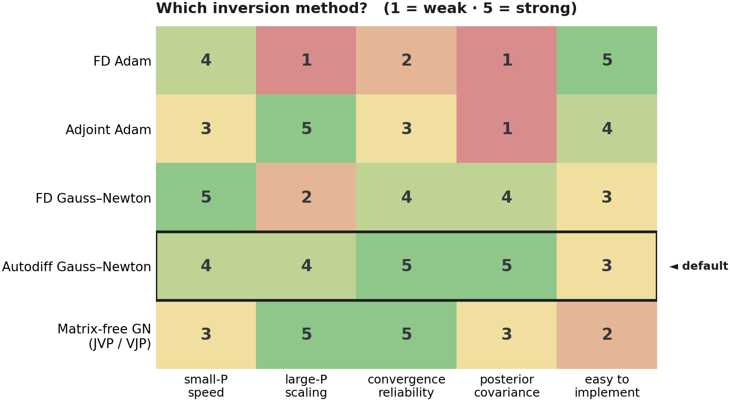
The full decision matrix behind the recommendations above — five algorithm families scored on small-P speed, large-P scaling, convergence reliability, posterior usefulness, and implementation effort.

Takeaway

The adjoint used to be the hardest, most artisanal part of quantitative Earth science — a thing you built once, carefully, and then guarded. Differentiable programming turned it into infrastructure: invisible, reliable, one line long.

That doesn’t make the science easier. Deciding what to invert, which observations to trust, how to regularise, where the model is lying to you — all of that is exactly as hard as it ever was. But we no longer pay a tax of two years and a thousand lines of hand-written derivative code just to get in the door. The gradient is free now. Go spend it on something interesting.

The JAX experiments and figures in this post were built in a scratch coding session with an AI assistant. More about the author at sudshu.github.io.

The views and opinions expressed in this article are those of the author alone and do not reflect those of the JPL, NASA and CALTECH.

Further reading

Adjoints and variational data assimilation

• Errico (1997), What is an adjoint model? Bull. Amer. Meteor. Soc. — doi
• Talagrand & Courtier (1987), Variational assimilation of meteorological observations with the adjoint vorticity equation. I: Theory. QJRMS — doi
• Giering & Kaminski (1998), Recipes for adjoint code construction. ACM TOMS — doi

Inverse modelling of the carbon cycle and methane

• Enting (2002), Inverse Problems in Atmospheric Constituent Transport. Cambridge Univ. Press — doi
• Gurney et al. (2002), Towards robust regional estimates of CO₂ sources and sinks using atmospheric transport models. Nature — doi
• Rödenbeck et al. (2003), CO₂ flux history 1982–2001 inferred from atmospheric data using a global inversion of atmospheric transport. ACP — doi
• Chevallier et al. (2005), Inferring CO₂ sources and sinks from satellite observations: method and application to TOVS data. JGR — doi
• Basu et al. (2013), Global CO₂ fluxes estimated from GOSAT retrievals of total column CO₂ — among the first global CO₂ flux inversions from GOSAT retrievals. ACP — doi
• Henze et al. (2007), Development of the adjoint of GEOS-Chem. ACP — doi
• Meirink et al. (2008), Four-dimensional variational data assimilation for inverse modelling of atmospheric methane emissions: method and comparison with synthesis inversion. ACP — doi
• Bergamaschi et al. (2009), Inverse modeling of global and regional CH₄ emissions using SCIAMACHY satellite retrievals. JGR — doi
• Bousquet et al. (2006), Contribution of anthropogenic and natural sources to atmospheric methane variability. Nature — doi

Remote sensing and satellite methane

• Veefkind et al. (2012), TROPOMI on the ESA Sentinel-5 Precursor: a GMES mission for global observations of the atmospheric composition for climate, air quality and ozone layer applications. Remote Sens. Environ. — doi
• Jacob et al. (2016), Satellite observations of atmospheric methane and their value for quantifying methane emissions. ACP — doi

My own, in this lineage

• Pandey et al. (2015), On the use of satellite-derived CH₄:CO₂ columns in a joint inversion of CH₄ and CO₂ fluxes — the first paper of my PhD. ACP — doi
• Pandey et al. (2019), Satellite observations reveal extreme methane leakage from a natural gas well blowout. PNAS — doi
• Pandey et al. (2022), Order of magnitude wall time improvement of variational methane inversions by physical parallelization: a demonstration using TM5-4DVAR. GMD — doi

Differentiable ML weather models

• Lam et al. (2023), Learning skillful medium-range global weather forecasting (GraphCast). Science — doi

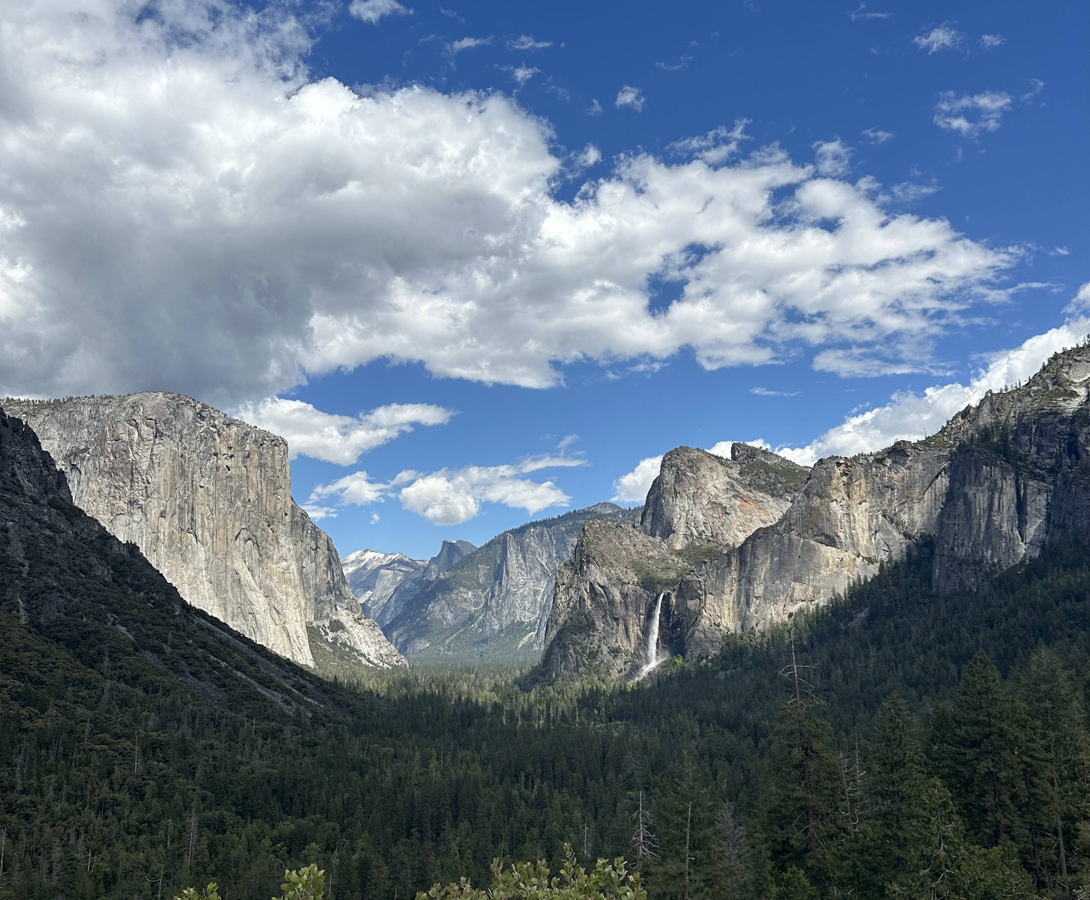
Yosemite Valley from the Wawona Tunnel View. The waterfall analysed in this post is Bridalveil Falls.

I went to Yosemite recently. It might be the most beautiful place I have ever visited. Standing in front of Bridalveil Falls, watching the water fall cleanly for a moment and then dissolve into spray, I noticed something: from far away, the waterfall looked almost steady. Up close, it was chaos — mist drifting sideways, white streaks appearing and disappearing, the same waterfall every second but never the same frame twice. I pulled out my phone and shot a 60-second clip of it to take home.

That made me wonder something concrete: when would a neural network be able to predict the next few moments of this waterfall better than a simple physics-based model? The real video itself is the ground truth. Both methods are scored on how closely their predicted frames match what actually happens next.

It is a tiny version of a bigger question now playing out in weather and climate science. Modern ML weather models can compete with physics-based forecasts, but they do so after learning from enormous archives of past weather. My waterfall experiment asks the same question at toy scale: how much data does ML need before it overtakes physics?

A few weekends of GPU time later, I have an answer. It is not “AI overtakes physics” once and for all — it is a crossover. Physics wins when data are scarce. ML wins once it has watched enough examples.

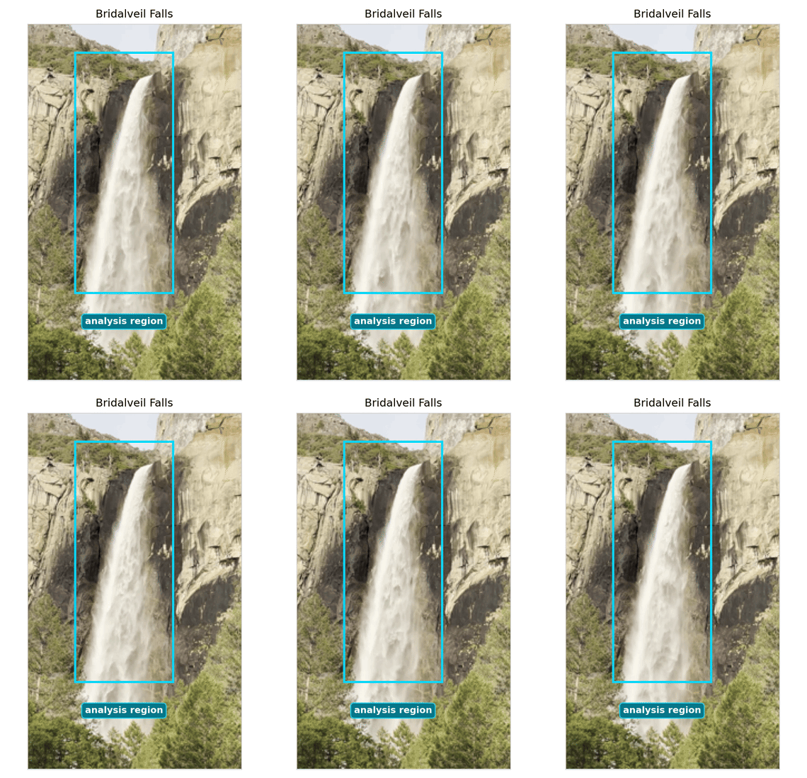
The clip. We focus on the boxed region — the cliff face, the falling column, and the mist envelope — and leave the static rocks and sky out of the comparison.

The prediction game

I gave both models the same game. Each model saw the last five video frames (the clip is 30 frames per second) and had to predict the next one. Then I made it harder: each prediction was fed back as input and the model had to predict the next one — and so on, for sixty steps. Two seconds of water that hasn’t happened yet.

The physics baseline estimated smooth motion in the image — an optical-flow field — and carried the waterfall forward by that motion. It starts with a useful built-in assumption: most of the water is moving continuously, mostly downward, under gravity.

The neural network learned from examples. It watched part of the clip during training, learned how the waterfall tends to change from one frame to the next, and then tried the same two-second rollout on a strictly held-out segment of the clip that it had never seen before.

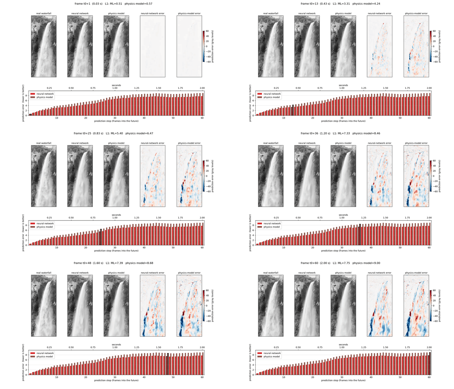
Here is what a 2-second forecast looks like, side by side. Real waterfall on the left, the two predictions in the middle, and per-frame prediction error in red and brown bars at the bottom.

Both methods blur as the rollout gets longer, which is expected: the turbulent details quickly become unpredictable. But with the full training clip, the neural network stays closer to the real waterfall than the physics baseline.

So the AI wins? Not quite.

The real result: how much data does ML need?

The interesting experiment wasn’t “can ML win?” It was “how much video does ML need before it wins?”

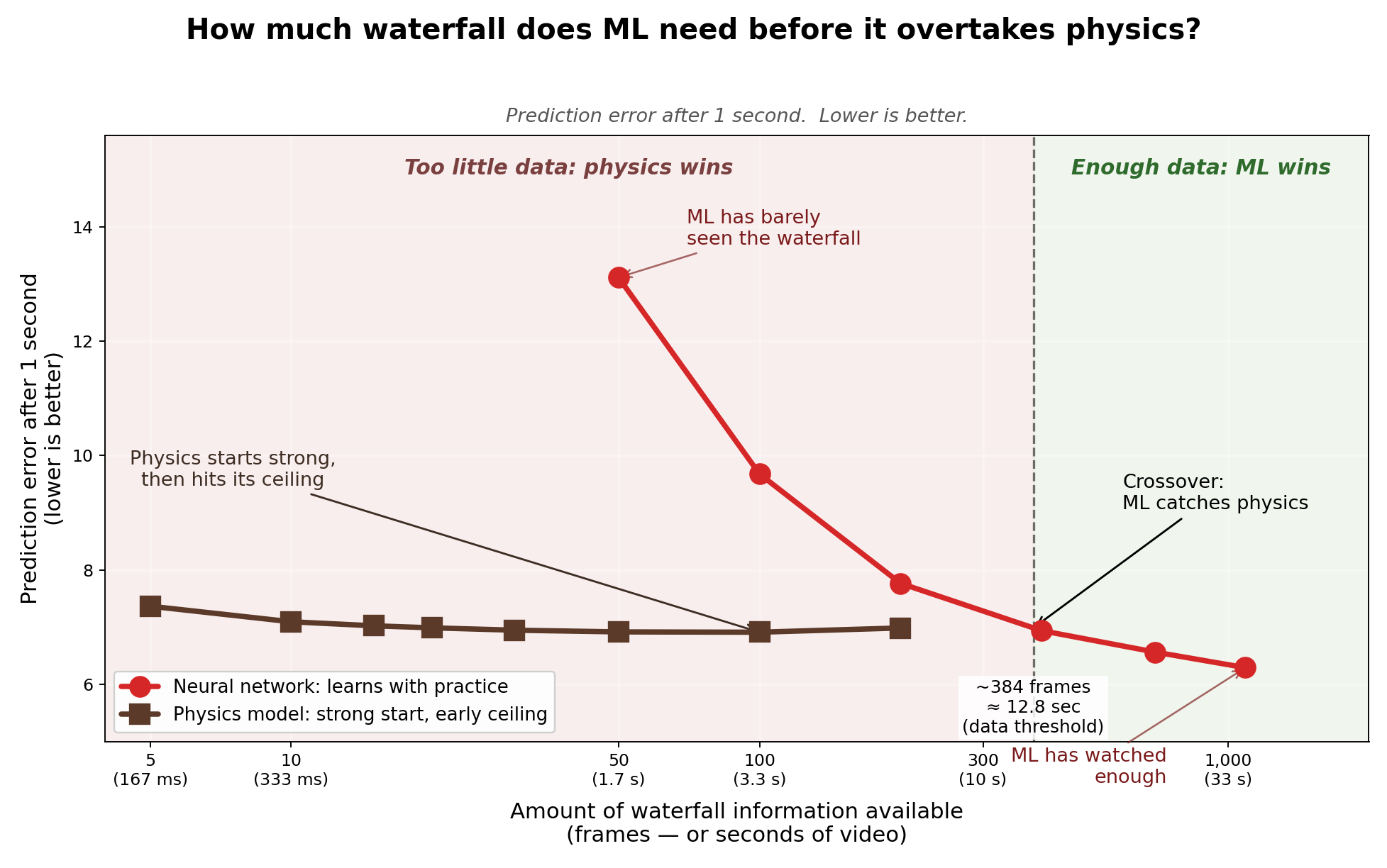
I retrained the neural network on different fractions of the clip — 50 frames, 100, 200, 400, 700, or all 1,090 — and re-ran the same forecast against the same physics model. This is what came out:

The data threshold. With 50 frames the neural network is much worse than the physics model. Around a few hundred frames — roughly 10 seconds of video — it catches up. With the whole clip, it wins.

This is the main result. The physics model has a ceiling; the neural network has a slope. The physics model starts strong because it already knows a useful rule: water moves smoothly and downward. But it cannot learn the messy residual structure of spray, flicker, and turbulence. The neural network starts with no such built-in knowledge — but with enough examples it learns the visual habits that smooth advection misses.

Why the crossover matters

The Yosemite waterfall is obviously not the atmosphere. But the shape of the result is familiar. Physics-based models encode strong assumptions and work immediately. ML models need data, but once enough data exist, they can learn structure that the simpler physics baseline misses.

That is why the training archive matters. ML weather models like Pangu-Weather, GraphCast, FourCastNet, and Aurora can compete with operational forecasts — but only after training on decades of ERA5 reanalysis. That archive is their version of the 300 frames of waterfall. When an ML weather model overtakes a physics-based forecast, the useful question is not only “which model won?” — it is also: how much data did the ML model need before it crossed over?

Caveats

• This is one clip of one waterfall. The exact crossover point could shift for a longer video, a different waterfall, or a different turbulent system.
• The physics model is intentionally simple — smooth optical-flow advection, not a full fluid-dynamics simulation. A full CFD model would be a different (and much more expensive) comparison.
• The neural network is also intentionally small and trained only on this clip. A larger pretrained video model would likely shift the curve, but the slope-versus-ceiling story would remain the point.

Nerdy note

• ML model. A 1.7-M-parameter Swin-UNet trained autoregressively with a short rollout curriculum (1 → 2 → 4 steps). It predicts a residual update rather than raw pixels: f̂(t+1) = clamp( f(t) + Δ , 0, 1 ). This helps because most pixels are nearly unchanged between adjacent frames; the useful signal is concentrated where the water and mist are actually moving.
• Physics baseline. A 4D-Var-style variational fit of a smooth velocity field to the past 5 frames, plus persistent-velocity advection of the most recent frame forward. This is “physics” in the limited sense of smooth image advection, not a full Navier-Stokes simulation. In bias-variance terms the physics baseline is high-bias (stable but restricted); the neural network is high-variance (data-hungry but improves with examples).
• Quantitative result. At a 1-second forecast lead time, the NWP-optimised physics baseline reaches L1 ≈ 7.32 (0–255 grayscale); the full-data ML model reaches L1 ≈ 6.29, about 14 % better. The crossover is best read as somewhere between 200 and 400 training frames, not a precise universal number.
• Code, video, and figures. github.com/sudshu/yosemite-waterfall-ml.

Takeaway

The lesson is not that ML magically overtakes physics. The lesson is that the winner depends on the data regime. With too little waterfall, the physics baseline wins because it starts with a useful prior. With enough waterfall, the neural network wins because it learns the messy structure that the simple physics model cannot represent.

Different systems, same question: where is the data threshold at which learning overtakes hand-built physics?

The coding was done using Claude Code. More about the author at sudshu.github.io.

The views and opinions expressed in this article are those of the author alone and do not reflect those of the JPL, NASA and CALTECH.