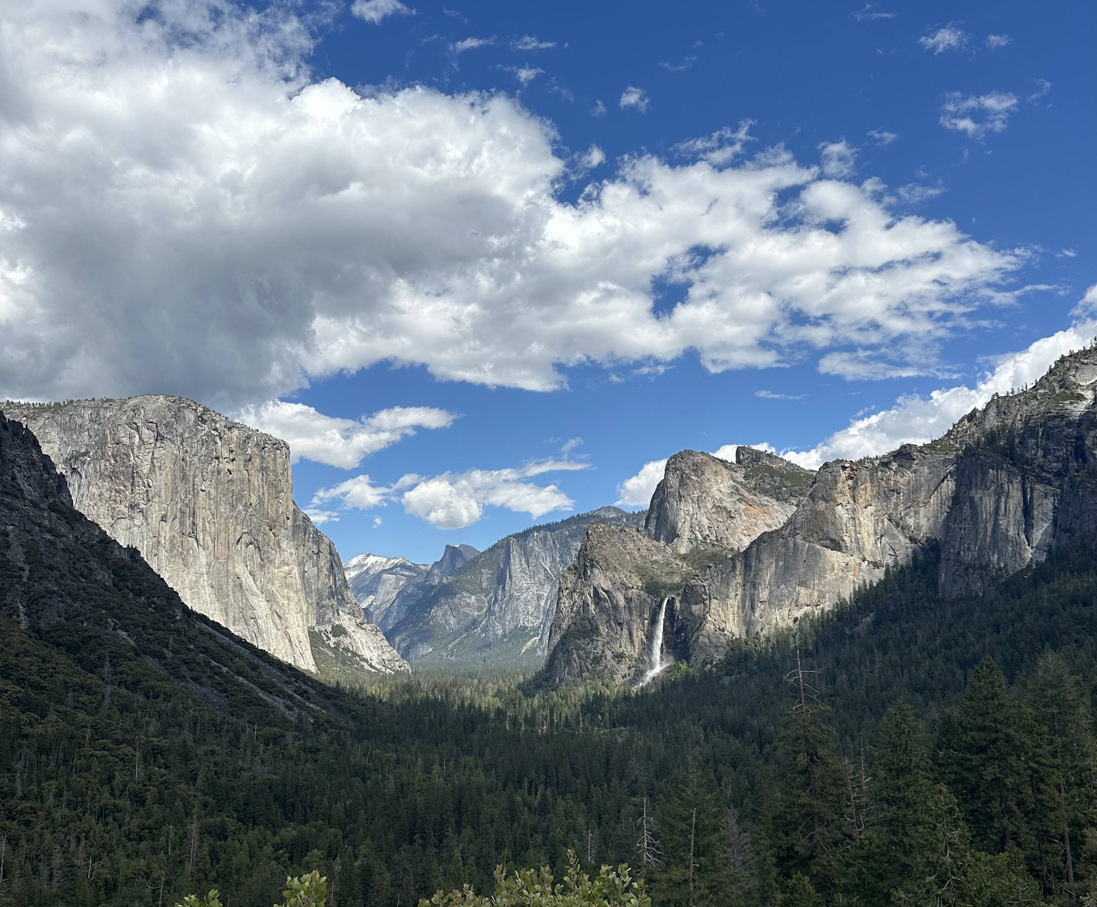
Yosemite Valley from the Wawona Tunnel View. The waterfall analysed in this post is Bridalveil Falls.
I went to Yosemite recently. It might be the most beautiful place I have ever visited. Standing in front of Bridalveil Falls, watching the water fall cleanly for a moment and then dissolve into spray, I noticed something: from far away, the waterfall looked almost steady. Up close, it was chaos — mist drifting sideways, white streaks appearing and disappearing, the same waterfall every second but never the same frame twice. I pulled out my phone and shot a 60-second clip of it to take home.
That made me wonder something concrete: when would a neural network be able to predict the next few moments of this waterfall better than a simple physics-based model? The real video itself is the ground truth. Both methods are scored on how closely their predicted frames match what actually happens next.
It is a tiny version of a bigger question now playing out in weather and climate science. Modern ML weather models can compete with physics-based forecasts, but they do so after learning from enormous archives of past weather. My waterfall experiment asks the same question at toy scale: how much data does ML need before it overtakes physics?
A few weekends of GPU time later, I have an answer. It is not “AI overtakes physics” once and for all — it is a crossover. Physics wins when data are scarce. ML wins once it has watched enough examples.
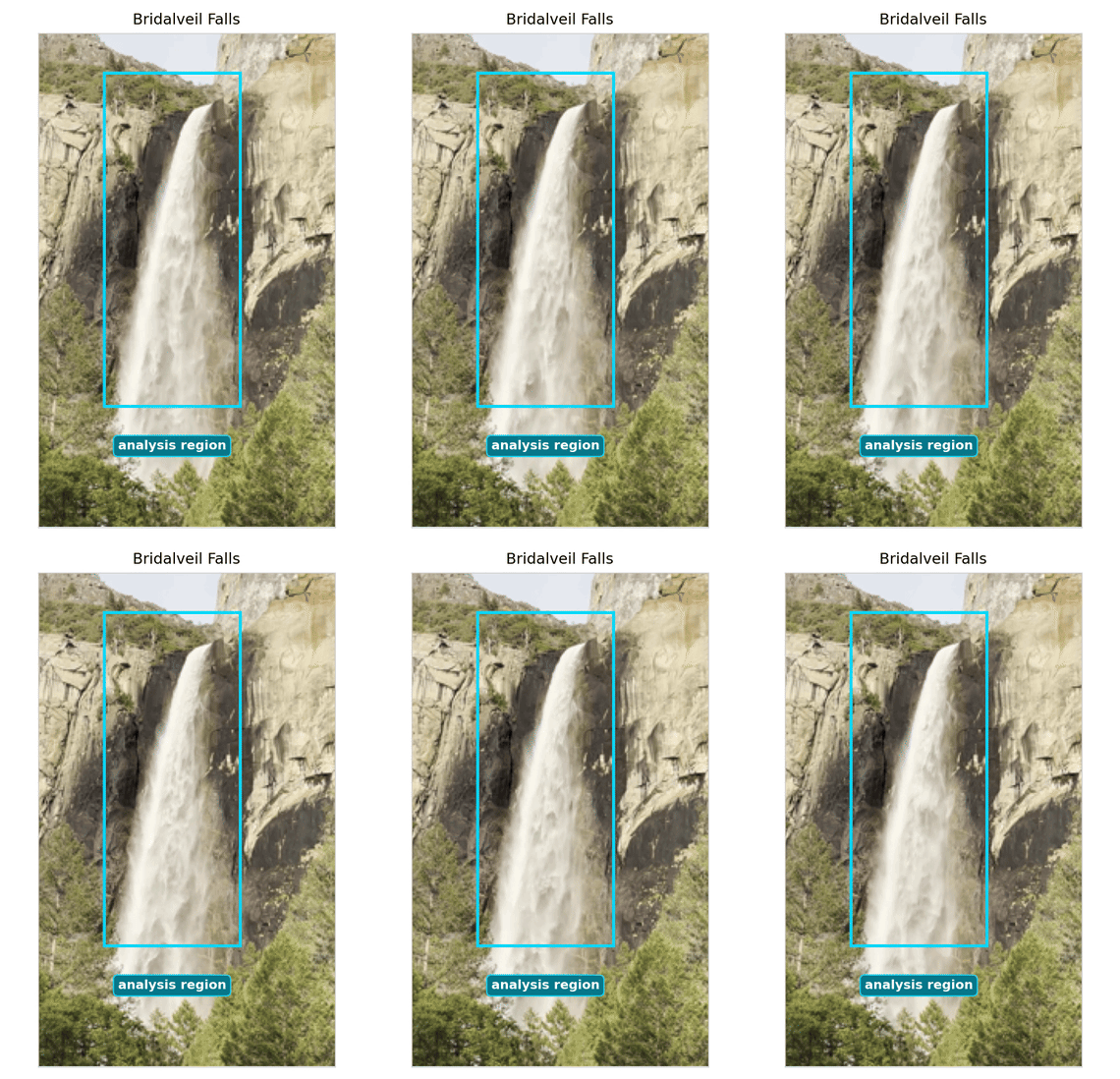
The clip. We focus on the boxed region — the cliff face, the falling column, and the mist envelope — and leave the static rocks and sky out of the comparison.
The prediction game
I gave both models the same game. Each model saw the last five video frames (the clip is 30 frames per second) and had to predict the next one. Then I made it harder: each prediction was fed back as input and the model had to predict the next one — and so on, for sixty steps. Two seconds of water that hasn’t happened yet.
The physics baseline estimated smooth motion in the image — an optical-flow field — and carried the waterfall forward by that motion. It starts with a useful built-in assumption: most of the water is moving continuously, mostly downward, under gravity.
The neural network learned from examples. It watched part of the clip during training, learned how the waterfall tends to change from one frame to the next, and then tried the same two-second rollout on a strictly held-out segment of the clip that it had never seen before.
Here is what a 2-second forecast looks like, side by side. Real waterfall on the left, the two predictions in the middle, and per-frame prediction error in red and brown bars at the bottom.
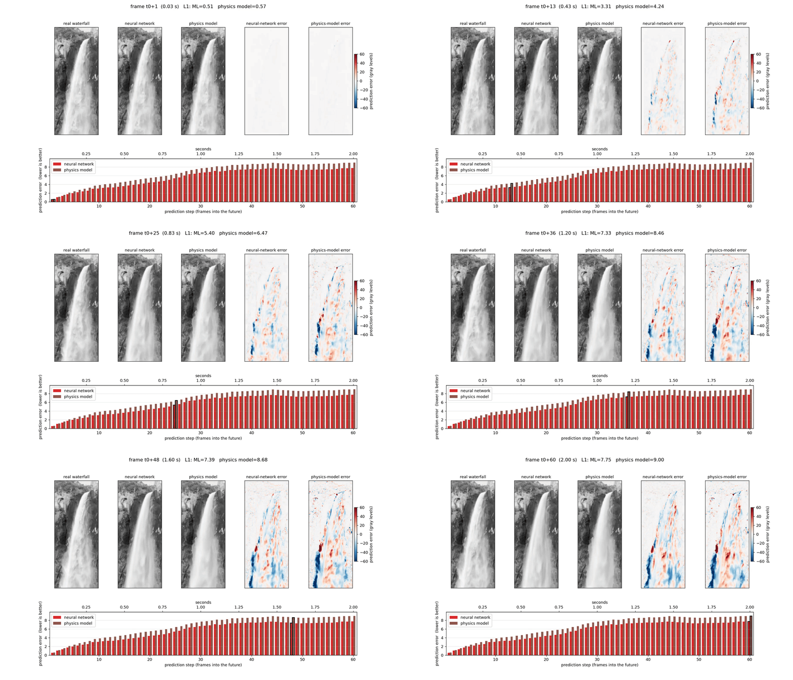
Both methods blur as the rollout gets longer, which is expected: the turbulent details quickly become unpredictable. But with the full training clip, the neural network stays closer to the real waterfall than the physics baseline.
So the AI wins? Not quite.
The real result: how much data does ML need?
The interesting experiment wasn’t “can ML win?” It was “how much video does ML need before it wins?”
I retrained the neural network on different fractions of the clip — 50 frames, 100, 200, 400, 700, or all 1,090 — and re-ran the same forecast against the same physics model. This is what came out:
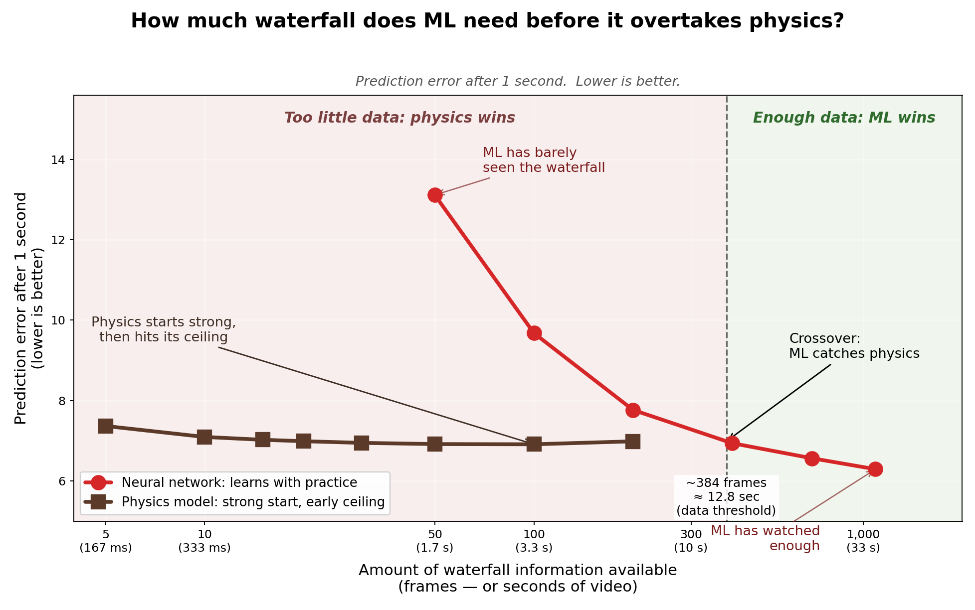
The data threshold. With 50 frames the neural network is much worse than the physics model. Around a few hundred frames — roughly 10 seconds of video — it catches up. With the whole clip, it wins.
This is the main result. The physics model has a ceiling; the neural network has a slope. The physics model starts strong because it already knows a useful rule: water moves smoothly and downward. But it cannot learn the messy residual structure of spray, flicker, and turbulence. The neural network starts with no such built-in knowledge — but with enough examples it learns the visual habits that smooth advection misses.
Why the crossover matters
The Yosemite waterfall is obviously not the atmosphere. But the shape of the result is familiar. Physics-based models encode strong assumptions and work immediately. ML models need data, but once enough data exist, they can learn structure that the simpler physics baseline misses.
That is why the training archive matters. ML weather models like Pangu-Weather, GraphCast, FourCastNet, and Aurora can compete with operational forecasts — but only after training on decades of ERA5 reanalysis. That archive is their version of the 300 frames of waterfall. When an ML weather model overtakes a physics-based forecast, the useful question is not only “which model won?” — it is also: how much data did the ML model need before it crossed over?
Caveats
- This is one clip of one waterfall. The exact crossover point could shift for a longer video, a different waterfall, or a different turbulent system.
- The physics model is intentionally simple — smooth optical-flow advection, not a full fluid-dynamics simulation. A full CFD model would be a different (and much more expensive) comparison.
- The neural network is also intentionally small and trained only on this clip. A larger pretrained video model would likely shift the curve, but the slope-versus-ceiling story would remain the point.
Nerdy note
- ML model. A 1.7-M-parameter Swin-UNet
trained autoregressively with a short rollout curriculum
(1 → 2 → 4 steps). It predicts a residual update rather than raw pixels:
f̂(t+1) = clamp( f(t) + Δ , 0, 1 ). This helps because most pixels are nearly unchanged between adjacent frames; the useful signal is concentrated where the water and mist are actually moving. - Physics baseline. A 4D-Var-style variational fit of a smooth velocity field to the past 5 frames, plus persistent-velocity advection of the most recent frame forward. This is “physics” in the limited sense of smooth image advection, not a full Navier-Stokes simulation. In bias-variance terms the physics baseline is high-bias (stable but restricted); the neural network is high-variance (data-hungry but improves with examples).
- Quantitative result. At a 1-second forecast lead time, the NWP-optimised physics baseline reaches L1 ≈ 7.32 (0–255 grayscale); the full-data ML model reaches L1 ≈ 6.29, about 14 % better. The crossover is best read as somewhere between 200 and 400 training frames, not a precise universal number.
- Code, video, and figures. github.com/sudshu/yosemite-waterfall-ml.
Takeaway
The lesson is not that ML magically overtakes physics. The lesson is that the winner depends on the data regime. With too little waterfall, the physics baseline wins because it starts with a useful prior. With enough waterfall, the neural network wins because it learns the messy structure that the simple physics model cannot represent.
Different systems, same question: where is the data threshold at which learning overtakes hand-built physics?
The coding was done using Claude Code. More about the author at sudshu.github.io.
The views and opinions expressed in this article are those of the author alone and do not reflect those of the JPL, NASA and CALTECH.